2013 Salary Survey

–Thanks to Stephen Kwok at the Tufts Laser Cytometry Flow Core at Tufts Medical School for conducting a flow cytometry salary survey last year, the results were posted to the Purdue list but have since been removed, so we are posting it here for anyone that is interested. I’ll also link it from the “Job Board” page.

2013 Flow Cytometry Survey

–There is a new category in the menu bar for “Humor” so that the feed does not end up with jokes overwhelming the “scholarly” posts or announcements. Feedback appreciated!

Posted in Uncategorized | Leave a comment

One of these things is not like the others…

For those of you that grew up with Sesame Street:
Three of these things belong together
Three of these things are kind of the same
Can you guess which one of these doesn’t belong here?
Now it’s time to play our game (time to play our game).

things1

Click here for the answer!

Posted in Humor | Leave a comment

Please join us for the 2013 annual New England Cytometry meeting on Tuesday November 5!

Visit the meetings page for details and the itinerary:
https://newenglandcytometry.com/meetings/2013-new-england-cytometry-user-group-meeting/

Credit cards now accepted for registration!
Click here to register!

It promises to be another excellent meeting, looking forward to seeing you there!

Posted in Uncategorized | Leave a comment

A clone by any other name…

BV421

Posted in Uncategorized | 1 Comment

Bee-ah-core or Bye-ah-core?

We have a Biacore 3000 from GE Healthcare, which uses Surface Plasmon Resonance technology (SPR) to perform label-free measurements of protein interactions, as well as detect differences in concentrations of solutions.  This technology can determine binding kinetics and protein interactions without the need for additional dyes or labels.  For the longest time I could NOT remember how to pronounce it, so I put together these slides to help me remember (and then went on to carry out the joke ad absurdum…):

biacore1

AND

biacore2

AND

biacorecore2

Posted in Humor | Leave a comment

FCS Files

xfilesflow is

Posted in Uncategorized | Leave a comment

Comp Comp

Compensation Comparison

I often hear of people looking at a compensation matrix and deciding if it is “good” or “bad”.  The actual values in themselves don’t give enough information to make this determination.  Voltages can be set to give you almost any value for the compensation matrix, and spillover for a tandem can change over time as the reagent breaks down, resulting in different “correct” compensation values (one comparison of spillover from PE-Cy5 into PE was 45% for an old vial of reagent, vs 7% for an unopened one of the same lot at the same settings).

There is a stigma in flow against high compensation values, and their validity is called into question. ISAC 2010 had a session about minimizing the compensation values for a panel, which some saw as a useless exercise.  From what I understand, this bias against high compensation is mostly a holdover from the early days of flow when compensation was done with pulse subtraction–a circuit would create a negative pulse proportional to the signal pulse in the primary channel to reduce the signal in the spillover channel and adjust for the spectral overlap. With small amounts of spillover this worked fine, but as you tried to compensate higher and higher values, it would be less accurate.

With the new digital systems today, the entire signal from each detector is quantified, and then compensation is applied mathematically. Depending on your system setup, it is possible that you could have greater than 100% compensation, meaning your signal in a spillover channel is higher than in your primary channel.  This can still be valid, even though Diva gives an error message when that happens. Causes for this include 1.The “spillover” detector is set to a higher voltage, so that even if more photons are reaching the primary detector, the spillover detector gives a higher output, or 2.The primary detector has a very narrow bandpass filter, and/or the spillover channel has a very wide filter, so that more photons are actually reaching the spillover detector. While these conditions are not optimal, there is nothing incorrect about them.  We are interested in identifying positive and negative events, so you could look at GFP in the “PE” detector and identify GFP positives, or some other non-optimal setup as long as you can get that separation, and it is still valid.

If you have FITC and PE single positive beads with negative beads, properly compensated, and look at histograms of FITC at a constant voltage, compared with PE over a range of voltages, the FITC signals are largely unaffected, while the PE+ is still identifiable over the full range, and just the separation changes:

compcomp5

If you look at the compensation values, you will find a wide range,

FITC/PE 400/400 400/500 400/550 400/600
PE- %FITC 16.4 82.9 165.4 315
FITC-%PE 2.9 0.5 0.3 0.2

Even at 315% compensation (bottom panel), the peaks are identifiable and still separated in the histogram, but looking at dot plots can reveal more.  At “normal” settings that give low spillover values, populations look normal–uncompensated on the left, compensated on the right, the red line being the boundary for “100% spillover”:

compcomp34

What can be observed at unbalanced settings is that events with a high signal in a given channel due to autofluorescence (or some other signal besides the fluor being compensated) can start to look strange when compensation percentages are very high—their high signal is NOT due to the fluor being compensated, so that “compensation” on those events is not accurate, and those bright autofluorescent populations will shift and cause strange plots:

compcomp12

The “bright” autofluorescent shift down disproportionately at such high values, becoming inverted.  So while compensation above 100% can be valid, it can start to cause some artifacts and aberrations in your plots.

High compensation values are an indication that your signals are high in another channel—this may be normal! Cy5 is excited by the 640 laser, and emits around 660, so PE-Cy5 has high spillover in the APC channel.  When you have high spillover values, take it as a warning that your sensitivity for double positives in that spillover channel will be reduced.  If your filter choices are optimized, you should be able to get the highest signal in the channel where you are measuring the fluorochrome of interest.  Keeping the values below 100% is still preferred, to avoid distorting the negative populations, but as long as you have sufficient separation of your populations of interest, you should be able to get reliable data.

Posted in Uncategorized | Leave a comment

You have chosen… poorly

It was brought to my attention that the filter on our 3 laser LSR2 might not be optimal for the AmCyan channel (490/40 bandpass, also used for Horizon V500, CFP, Aqua Live/Dead dye, and Q525)–it was centered on the peak of Amcyan, but might also pick up stray light from the 488 laser. After some testing, I discovered that this was indeed true, as the image below shows (click to enlarge).

I used 6 peak beads and set the brightest bead to 10^5.  Plot 1 shows the 490/40 filter, notice the high signal for the lowest peak, “P2”. Using a 525/50 to avoid the 488 region (plot 2) you can see the dimmest bead has much greater separation from the next peak “P3”, in fact 4 times the separation based on a ratio of the means. I repeated the measurements setting the brightest peak to 10e4 instead of 10e5, and while the difference is not as evident visually (plots 3 and 4), mathematically it is again a 4-fold difference.

To show it is indeed due to the blue laser, I then used APC as the threshold parameter and blocked the blue laser to generate plot 5, and saw a 2-fold improvement compared to the same settings with the laser on, so there is still some spillover of light from the blue laser.

At least running with the wrong filter didnt turn me to dust, like this guy that also “chose…poorly”

http://www.youtube.com/watch?v=qOajmNKsb5Q

Posted in Uncategorized | Leave a comment

Staying focused….

Just a quick post since we are in the midst of relocating to a new facility…

hydrodynamicfocusing

Posted in Uncategorized | Leave a comment

As bright or brighter…

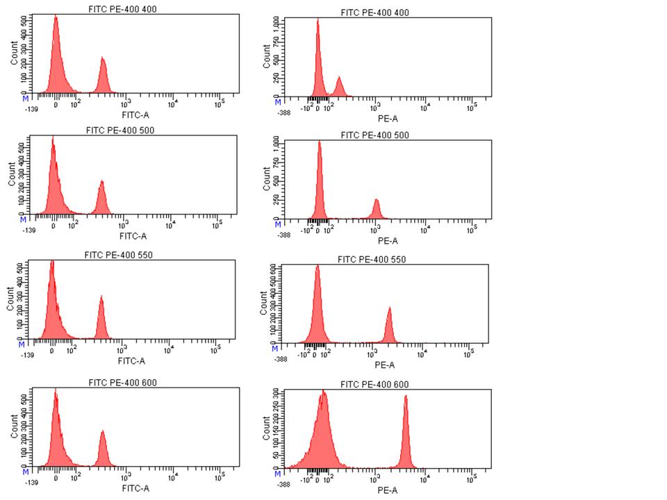
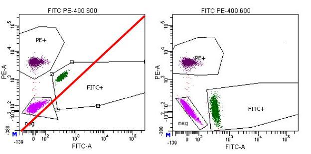
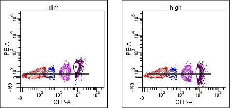
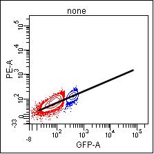
So the earlier posts were a lead-in to this one, which I hope will clarify this important issue in compensation.  When calculating compensation, it is important to make sure that your single stained control is as bright or brighter than your experimental sample for each color.  To illustrate why this is important, a GFP+ sample was measured in 6 detectors off of the blue laser:  525/50 to measure the GFP, and then also in 576/26 (PE), 610/20 (PE-TR), 675/20 (PE-Cy5), 695/40 (PE-Cy5.5), and 780/60 (PE-Cy7) to examine the spillover of GFP into these other detectors.  Populations are identified based on their GFP signal (neg, dim, mid, and bright), and plot titles refer to what was used to determine compensation from each channel (none=no compensation, then dim, mid, or high/bright indicates which population was compared to neg to calculate spillover).abob01

Compensation is basically determining the ratio of the two detectors in question: the signal in the primary detector, and then how much signal is detected in another channel (the spillover channel) for that intensity of staining.  This allows the researcher to subtract the spillover signal from other channels so that signal from that detector corresponds to that additional parameter.  In essence, the slope of the population’s signals is what is being determined:


abob02
If you are using a dim population, noise in the detection system reduces your sensitivity and so the signal will not be accurately measured.  When you look at a brighter population, it will probably not be compensated accurately.

abob03

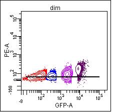
Compensating with the dim population, the resulting means are neg 57, dim 57, mid 89, and bright 182.

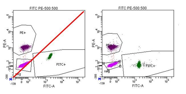
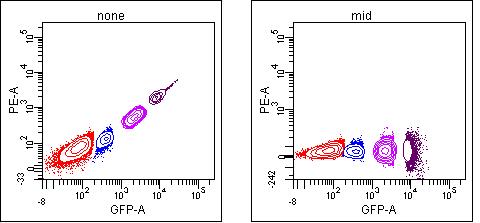
In the case of a high spillover between channels, such as GFP spilling into the PE channel, it is possible to get decent compensation of the bright population using the “mid” population, since the signal is high enough to give you a more accurate measurement:

abob04
mean: 56, 52, 57, 49

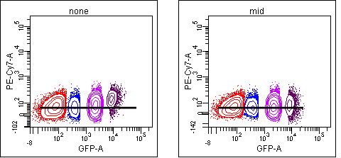
But this may not be true for other spillovers in the same panel.  As you move further away from the optimal detector for that fluorochrome, only the brightest events will show spillover that can be detected above background:

abob05

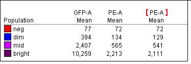
In this case, using the “mid” population results in slight undercompensation of the brights (means of 72, 72, 73, 89) even though it “looks” ok.  (Of course, you should never use visualization to set compensation, but compare the means or medians of the negative and positive populations).

Even if different spillover values are generated using bright vs dim populations, the bright values will still work for the dim.  Changes in the spillover values have a much greater impact on events with high signal than dim.  For comparison, a 1% change in compensation in this example changes the mean signal of the dim by 5, mid by 24, or bright by 102 units in the spillover channel:

abob06

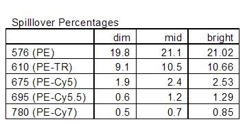
Correcting the spillover from 19.8% using the dim, which leads to the bright being undercompensated by 125 (73% off), to 21.02% using the bright makes the dim “overcompensated” by 4 which is hardly noticeable (5.5% off).

abob07

And just for completeness, below are tables of the spillover % for the different setups:abob08

…And the statistics tables for the means (none, dim, mid, bright)

abob09

Posted in Uncategorized | Tagged , | Leave a comment