posted by Mike Waring

In the course of running experiments in Diva, you may have found that your negative population ends up well below 0. This came up in a Purdue post in 2009 and Mario Roederer gave an in-depth explanation (https://lists.purdue.edu/pipermail/cytometry/2009-June/037462.html). I’ve put together a write-up with pictures that I share with my users and thought it would be helpful to post it here.

Baseline Correction and potential issues

In order to remove background signals due to unbound fluorophores, dark current, and ambient light, the Diva Software averages signals between events and subtracts this from the total signal. If there is no signal for that parameter, this can result in a negative value for that event.

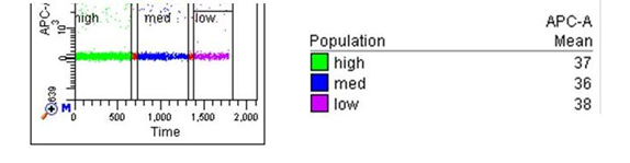
Most of the time, signals are corrected appropriately and this results in a population mean that is consistent regardless of flow rate. (You may possibly see a higher CV/more spread at higher flow rate due to greater measurement error). Population labels to the right refer to the flow rate used for acquisition of the events in that gate.

        

Where it can go wrong

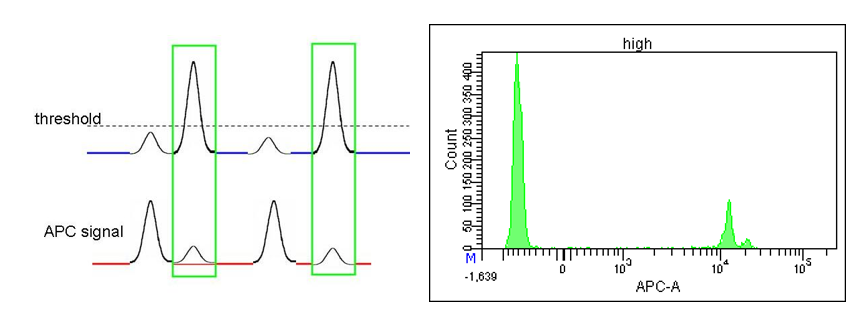
          Usually threshold is set on FSC– in cases where particles are very different in size, one may be below threshold while the other is on scale (such as cells vs. beads or debris).
Because it is below threshold and is not an “event”, the fluorescent signal of the small particle is averaged into the baseline and subtracted from the signals.
In this example, negative cells and fluorescent beads are in the same sample.  The beads are so small they fall below FSC threshold and are ignored.  Their bright fluorescent signal is averaged into the “baseline” which is subtracted from the signal measurement
This can lead to your negative populations shifting artificially far into negative values and can lead to problems with your data files. Here the positive APC peak is either a bead that managed to generate FSC above threshold, or stuck to a cell.

Confirming issue:

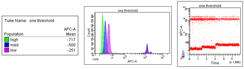
One way this issue can be illustrated is to run at different flow rates.  The higher the flow rate, the more “undetected” particles that will be present, and the higher the baseline error so the further into the negative your population will go. (If your population doesnt go further into the negative with higher flow rates, then it may be a compensation issue).

Solution:

One way to accommodate this is to apply a second threshold using the fluorescent parameter where the bright small particles are occurring (we often see it with PE antibodies that have aggregated):

Applying a second threshold that identifies the small particle based on fluorescence makes sure all events are detected and the baseline is not erroneously high—events above T1 OR T2 will be recognized and recorded. The large APC+ peak below consists of the beads being detected by fluorescence threshold: 

Alternatively, you can decrease your FSC threshold to include the debris, but you may not be able to set it low enough to detect all of them, or may end up in the FSC noise. This also defeats the purpose of a higher threshold being used to crop out unwanted debris events in the data file. Another option would be to set a “Save gate” using a FSC threshold, so that the small particles are recognized during acquisition but not saved in the data file.

From BD’s whitepages:
2.5 Baseline Restoration
PMT signals can contain a high level of background from a variety of sources: light from unbound fluorophores, PMT dark current, and ambient light. Background signal is eliminated in two stages. The first, gross adjustment is made during the initial conversion of the signal from current to pulse. (Photomultiplier tubes are a source of current.) After pulse conversion in the preamp, the output signal falls in the range of 0 to 5 V. This initial gross adjustment preserves the dynamic range of the A/D converters for signals of interest, and maintains a safety margin of 100 mV.
The second, final adjustment is made just before area and height are measured. The FPGAs (Figure 2) calculate a running average of the data outside any window gate to remove the last 100 mV (Figure 3).